Solving Nonlinear Equations

Let it be required to solve the equation

Where
is a nonlinear continuous function.

Methods for solving equations are divided into direct and iterative. Direct methods are methods that allow you to calculate a solution using a formula (for example, finding the roots of a quadratic equation). Iterative methods are methods in which some initial approximation is given and a converging sequence of approximations to the exact solution is constructed, with each subsequent approximation being calculated using the previous ones.

The complete solution of the problem can be divided into 3 stages:

Set the number, nature and location of the roots of equation (1).

Find approximate values ​​of the roots, i.e. indicate the gaps in which the roots will be found (separate the roots).

Find the value of the roots with the required accuracy (specify the roots).

There are various graphical and analytical methods for solving the first two problems.

The most illustrative method for separating the roots of equation (1) is to determine the coordinates of the intersection points of the graph of the function
with the abscissa axis. Abscissas graph intersection points
with axle
are the roots of equation (1)

The intervals of isolation of the roots of equation (1) can be obtained analytically, based on theorems on the properties of functions that are continuous on a segment.

If, for example, the function
continuous on the segment
And
, then according to the Bolzano-Cauchy theorem, on the segment
there is at least one root of equation (1) (an odd number of roots).

If the function
satisfies the conditions of the Bolzano-Cauchy theorem and is monotonic on this segment, then on
there is only one root of equation (1). Thus, equation (1) has on
the only root if the conditions are met:

If a function is continuously differentiable on a given interval, then we can use the corollary of Rolle's theorem, according to which there is always at least one stationary point between a pair of roots. The algorithm for solving the problem in this case will be as follows:

A useful tool for separating roots is also the use of Sturm's theorem.

The solution of the third problem is carried out by various iterative (numerical) methods: the dichotomy method, the simple iteration method, Newton's method, the chord method, etc.

Example Let's solve the equation
method simple iteration. Let's set
. Let's build a graph of the function.

The graph shows that the root of our equation belongs to the segment
, i.e.
is the isolation segment of the root of our equation. Let us check this analytically, i.e. fulfillment of conditions (2):

Recall that the original equation (1) in the simple iteration method is transformed to the form
and iterations are carried out according to the formula:

(3)

Performing calculations according to formula (3) is called one iteration. The iterations stop when the condition is met
, where is the absolute error in finding the root, or
, where -relative error.

The simple iteration method converges if the condition
for
. Function selection
in formula (3) for iterations, one can influence the convergence of the method. In the simplest case
with a plus or minus sign.

In practice, it is often expressed
directly from equation (1). If the convergence condition is not met, it is converted to the form (3) and selected. We represent our equation in the form
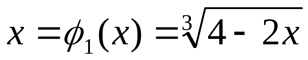(we express x from the equation). Let's check the convergence condition of the method:

for
. Note that the convergence condition is not met
, so we take the root isolation segment
. In passing, we note that when representing our equation in the form
, the convergence condition of the method is not met:
on the segment
. The graph shows that
increases faster than the function
(|tg| angle of inclination of the tangent to
on the segment
)

Let's choose
. We organize iterations according to the formula:

We programmatically organize the process of iterations with a given accuracy:

> fv:=proc(f1,x0,eps)

> k:=0:

x:=x1+1:

while abs(x1-x)> eps do

x1:=f1(x):

print(evalf(x1,8)):

print(abs(x1-x)):

:printf("Number of iterations=%d ",k):

end:

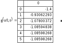
At iteration 19, we got the root of our equation

with absolute error

Let's solve our equation Newton's method. Iterations in Newton's method are carried out according to the formula:

Newton's method can be considered as a method of simple iteration with a function, then the convergence condition of Newton's method can be written as:

.

In our designation
and the convergence condition is satisfied on the segment
which can be seen on the graph:

Recall that Newton's method converges at a quadratic rate and the initial approximation must be chosen sufficiently close to the root. Let's do the calculations:
, initial approximation, . We organize iterations according to the formula:

We programmatically organize the process of iterations with a given accuracy. At 4 iterations, we get the root of the equation

from
We have considered methods for solving nonlinear equations using cubic equations as an example; naturally, various types of nonlinear equations are solved by these methods. For example, solving the equation

Newton's method with
, we find the root of the equation on [-1.5;-1]:

The task: Solve non-linear equations with accuracy

0.

bisecting a segment (dichotomy)

simple iteration.

Newton (tangent)

secant - chord.

Task options are calculated as follows: the list number is divided by 5 (
), the integer part corresponds to the equation number, the remainder to the method number.

General view of the nonlinear equation

f(x)=0, (6.1)

where is the function f(x) – is defined and continuous in some finite or infinite interval.

By type of function f(x) nonlinear equations can be divided into two classes:

Algebraic;

Transcendent.

Algebraic called equations containing only algebraic functions (entire, rational, irrational). In particular, a polynomial is an entire algebraic function.

transcendent called equations containing other functions (trigonometric, exponential, logarithmic, etc.)

Solve non-linear equation means to find its roots or root.

Any argument value X, reversing the function f(x) to zero is called the root of the equation(6.1) or function zero f(x).

6.2. Solution Methods

Methods for solving nonlinear equations are divided into:

Iterative.

Direct Methods allow us to write the roots in the form of some finite relation (formula). From the school algebra course, such methods are known for solving a quadratic equation, a biquadratic equation (the so-called simplest algebraic equations), as well as trigonometric, logarithmic, and exponential equations.

However, the equations encountered in practice cannot be solved by such simple methods, because

Function type f(x) can be quite complex;

Function coefficients f(x) in some cases they are known only approximately, so the problem of exact determination of the roots loses its meaning.

In these cases, to solve nonlinear equations, we use iterative methods that is, methods of successive approximations. The algorithm for finding the root of the equation, it should be noted isolated, that is, one for which there is a neighborhood that does not contain other roots of this equation, consists of two stages:

root separation, namely, the determination of the approximate value of the root or segment, which contains one and only one root.

refinement of approximate value root, that is, bringing its value to a given degree of accuracy.

At the first stage, the approximate value of the root ( initial approximation) can be found in various ways:

For physical reasons;

From the solution of a similar problem;

From other source data;

Graphic method.

Let's take a closer look at the last method. Real Equation Root

f(x)=0

can be approximately defined as the abscissa of the intersection point of the graph of the function y=f(x) with axle 0x. If the equation does not have roots close to each other, then in this way they are easily determined. In practice, it is often advantageous to replace equation (6.1) with the equivalent

f 1 (x)=f 2 (x)

where f 1 (x) And f 2 (x) - simpler than f(x) . Then, plotting the graphs of the functions f 1 (x) And f 2 (x), the desired root (roots) will be obtained as the abscissa of the intersection point of these graphs.

Note that the graphical method, for all its simplicity, is usually applicable only for a rough determination of the roots. Particularly unfavorable, in terms of loss of accuracy, is the case when the lines intersect at a very sharp angle and practically merge along a certain arc.

If such a priori estimates of the initial approximation cannot be made, then two closely spaced points are found a, b between which the function has one and only one root. For this action, it is useful to remember two theorems.

Theorem 1. If a continuous function f(x) takes values ​​of different signs at the ends of the segment [ a, b], i.e

f(a) f(b)<0, (6.2)

then inside this segment there is at least one root of the equation.

Theorem 2. The root of the equation on the interval [ a, b] will be unique if the first derivative of the function f’(x), exists and keeps a constant sign inside the segment, that is

(6.3)

Segment selection [ a, b] performed

Graphically;

Analytically (by examining the function f(x) or selection).

At the second stage, a sequence of approximate root values ​​is found X 1 , X 2 , … , X n. Each calculation step x i called iteration. If x i with increasing n approach the true value of the root, then the iterative process is said to converge.

Equations that contain unknown functions raised to a power greater than one are called non-linear.
For example, y=ax+b is a linear equation, x^3 - 0.2x^2 + 0.5x + 1.5 = 0 is non-linear (generally written as F(x)=0).

A system of nonlinear equations is the simultaneous solution of several nonlinear equations with one or more variables.

There are many methods solving nonlinear equations and systems of nonlinear equations, which are usually classified into 3 groups: numerical, graphical and analytical. Analytical methods make it possible to determine the exact values ​​of the solution of equations. Graphical methods are the least accurate, but allow in complex equations to determine the most approximate values, from which in the future you can begin to find more accurate solutions to the equations. The numerical solution of nonlinear equations involves passing through two stages: separation of the root and its refinement to a certain specified accuracy.
The separation of the roots is carried out in various ways: graphically, using various specialized computer programs, etc.

Let's consider several methods for refining roots with a specific accuracy.

Methods for the numerical solution of nonlinear equations

half division method.

The essence of the half division method is to divide the interval in half (с=(a+b)/2) and discard the part of the interval in which there is no root, i.e. condition F(a)xF(b)

Fig.1. Using the method of half division in solving nonlinear equations.

Consider an example.

Let's divide the segment into 2 parts: (a-b)/2 = (-1+0)/2=-0.5.
If the product F(a)*F(x)>0, then the beginning of the segment a is transferred to x (a=x), otherwise, the end of the segment b is transferred to the point x (b=x). We divide the resulting segment in half again, etc. All calculations are shown in the table below.

Fig.2. Calculation results table

As a result of calculations, we obtain the value, taking into account the required accuracy, equal to x=-0.946

chord method.

When using the chord method, a segment is specified, in which there is only one root with the specified accuracy e. A line (chord) is drawn through the points in the segment a and b, which have coordinates (x(F(a); y(F(b))). Next, the points of intersection of this line with the abscissa axis (point z) are determined.
If F(a)xF(z)

Fig.3. Using the method of chords in solving nonlinear equations.

Consider an example. It is necessary to solve the equation x^3 - 0.2x^2 + 0.5x + 1.5 = 0 to within e

In general, the equation looks like: F(x)= x^3 - 0.2x^2 + 0.5x + 1.5

Find the values ​​of F(x) at the ends of the segment :

F(-1) = - 0.2>0;

Let's define the second derivative F''(x) = 6x-0.4.

F''(-1)=-6.4
F''(0)=-0.4

At the ends of the segment, the condition F(-1)F’’(-1)>0 is observed, therefore, to determine the root of the equation, we use the formula:

All calculations are shown in the table below.

Fig.4. Calculation results table

As a result of calculations, we obtain the value, taking into account the required accuracy, equal to x=-0.946

Tangent Method (Newton)

This method is based on the construction of tangents to the graph, which are drawn at one of the ends of the interval. At the point of intersection with the X-axis (z1), a new tangent is built. This procedure continues until the obtained value is comparable with the desired accuracy parameter e (F(zi)

Fig.5. Using the method of tangents (Newton) in solving nonlinear equations.

Consider an example. It is necessary to solve the equation x^3 - 0.2x^2 + 0.5x + 1.5 = 0 to within e

In general, the equation looks like: F(x)= x^3 - 0.2x^2 + 0.5x + 1.5

Let's define the first and second derivatives: F'(x)=3x^2-0.4x+0.5, F''(x)=6x-0.4;

F''(-1)=-6-0.4=-6.4
F''(0)=-0.4
The condition F(-1)F''(-1)>0 is fulfilled, so the calculations are made according to the formula:

Where x0=b, F(a)=F(-1)=-0.2

All calculations are shown in the table below.

Fig.6. Calculation results table

As a result of calculations, we obtain the value, taking into account the required accuracy, equal to x=-0.946

Mathematics as a science arose in connection with the need to solve practical problems: measurements on the ground, navigation, etc. As a result, mathematics was numerical mathematics and its goal was to obtain a solution in the form of a number. The numerical solution of applied problems has always interested mathematicians. The largest representatives of the past combined in their studies the study of natural phenomena, obtaining their mathematical description, i.e. his mathematical model and his research. The analysis of complicated models required the creation of special, usually numerical methods for solving problems. The names of some of these methods indicate that they were developed by the largest scientists of their time. These are the methods of Newton, Euler, Lobachevsky, Gauss, Chebyshev, Hermite.

The present time is characterized by a sharp expansion of the applications of mathematics, largely associated with the creation and development of computer technology. As a result of the emergence of computers in less than 40 years, the speed of operations has increased from 0.1 operations per second with manual counting to 10 operations per second on modern computers.

The widespread opinion about the omnipotence of modern computers gives rise to the impression that mathematicians have got rid of all the troubles associated with the numerical solution of problems, and the development of new methods for solving them is no longer so significant. In reality, the situation is different, since the needs of evolution, as a rule, set before science tasks that are on the verge of its capabilities. The expansion of the application of mathematics led to the mathematization of various branches of science: chemistry, economics, biology, geology, geography, psychology, medicine, technology, etc.

There are two circumstances that initially led to the desire for the mathematization of sciences:

firstly, only the use of mathematical methods makes it possible to give a quantitative character to the study of one or another phenomenon of the material world;

secondly, and this is the main thing, only the mathematical way of thinking makes an object. This method of research is called a computational experiment - the study is fully objective.

IN Lately there is another factor that has a strong impact on the processes of mathematization of knowledge. This is the rapid development of computer technology. The use of computers for solving scientific, engineering, and applied problems in general is entirely based on their mathematization.

Mathematical models.

Modern technology for the study of complex problems is based on the construction and analysis, usually with the help of a computer, of mathematical models of the problem being studied. Usually, a computational experiment, as we have already seen, consists of a number of stages: setting a problem, building a mathematical model (mathematical formulation of the problem), developing a numerical method, developing an algorithm for implementing a numerical method, developing a program, debugging a program, performing calculations, analyzing results.

So, the use of computers for solving any scientific or engineering problem is inevitably associated with the transition from a real process or phenomenon to its mathematical model. Thus, the use of models in scientific research and engineering practice is the art of mathematical modeling.

A model is usually called a represented or materially realized system that reproduces the main most significant features of a given phenomenon.

The main requirements for the mathematical model are the adequacy of the phenomenon under consideration, i.e. it should adequately reflect character traits phenomena. At the same time, it should have comparative simplicity and accessibility of research.

The mathematical model reflects the dependence between the conditions for the occurrence of the phenomenon under study and its results in certain mathematical constructions. The most commonly used structures are: mathematical concepts Keywords: function, functional, operator, numerical equation, ordinary differential equation, partial differential equation.

Mathematical models can be classified according to different criteria: static and dynamic, concentrated and distributed; deterministic and probabilistic.

Consider the problem of finding roots nonlinear equation

The roots of equation (1) are those values ​​of x that, when substituting, turn it into an identity. Only for the simplest equations it is possible to find a solution in the form of formulas, i.e. analytical form. More often it is necessary to solve equations by approximate methods, the most widespread among which, in connection with the advent of computers, are numerical methods.

The algorithm for finding roots by approximate methods can be divided into two stages. At the first, the location of the roots is studied and their separation is carried out. There is an area in which there is a root of the equation or an initial approximation to the root x 0 . The simplest way The solution to this problem is to study the graph of the function f(x) . In the general case, to solve it, it is necessary to involve all means of mathematical analysis.

The existence on the found interval of at least one root of equation (1) follows from the Bolzano condition:

f(a)*f(b)<0 (2)

It is also assumed that the function f(x) is continuous on the given segment. However, this condition does not answer the question about the number of roots of the equation on a given interval. If the requirement of continuity of the function is supplemented with the requirement of its monotonicity, and this follows from the sign-constancy of the first derivative, then we can assert the existence of a unique root on a given segment.

When localizing roots, it is also important to know the basic properties of this type of equation. For example, recall some properties of algebraic equations:

where are real coefficients.

• a) An equation of degree n has n roots, among which there can be both real and complex ones. Complex roots form complex conjugate pairs and, therefore, the equation has an even number of such roots. For an odd value of n, there is at least one real root.
• b) The number of positive real roots is less than or equal to the number of variable signs in the sequence of coefficients. Replacing x with -x in equation (3) allows you to estimate the number of negative roots in the same way.

At the second stage of solving equation (1), using the obtained initial approximation, an iterative process is constructed that makes it possible to refine the value of the root with some predetermined accuracy. The iterative process consists in successive refinement of the initial approximation. Each such step is called an iteration. As a result of the iteration process, a sequence of approximate values ​​of the roots of the equation is found. If this sequence approaches the true value of the root x as n grows, then the iterative process converges. An iterative process is said to converge to at least order m if the following condition is satisfied:

where С>0 is some constant. If m=1 , then one speaks of first-order convergence; m=2 - about quadratic, m=3 - about cubic convergence.

The iterative cycles end if, for a given permissible error, the criteria for absolute or relative deviations are met:

or the smallness of the residual:

This work is devoted to the study of an algorithm for solving nonlinear equations using Newton's method.

There are many different methods for solving nonlinear equations, some of them are presented below:

• 1)Iteration Method. When solving a non-linear equation by iteration, we use the equation in the form x=f(x). The initial value of the argument x 0 and the accuracy e are given. The first approximation of the solution x 1 is found from the expression x 1 \u003d f (x 0), the second - x 2 \u003d f (x 1), etc. In the general case, the i+1 approximation is found by the formula xi+1 =f(xi). We repeat this procedure until |f(xi)|>e. The condition for the convergence of the iteration method |f"(x)|
• 2)Newton's method. When solving a nonlinear equation by the Newton method, the initial value of the argument x 0 and the accuracy e are set. Then, at the point (x 0, F (x 0)) we draw a tangent to the graph F (x) and determine the intersection point of the tangent with the abscissa axis x 1. At the point (x 1, F (x 1)) we again build a tangent, find the next approximation of the desired solution x 2, etc. We repeat this procedure until |F(xi)| > e. To determine the point of intersection (i + 1) of the tangent with the abscissa axis, we use the following formula

x i+1 \u003d x i -F (x i) F "(x i).

Convergence condition for the tangent method F(x 0) F""(x)>0, etc.

3). dichotomy method. The solution technique is reduced to the gradual division of the initial uncertainty interval in half according to the formula

C to \u003d a to + in to / 2.

In order to choose the necessary one from the two resulting segments, it is necessary to find the value of the function at the ends of the resulting segments and consider the one on which the function will change its sign, that is, the condition f (a k) * f (in k)<0.

The process of dividing the segment is carried out until the length of the current uncertainty interval is less than the specified accuracy, that is, in k - a k< E. Тогда в качестве приближенного решения уравнения будет точка, соответствующая середине интервала неопределённости.

4). chord method. The idea of ​​the method is that a chord is constructed on the segment that contracts the ends of the arc of the graph of the function y=f(x), and the point c, the intersection of the chord with the abscissa axis, is considered an approximate value of the root

c = a - (f(a) x (a-b)) / (f(a) - f(b)),

c \u003d b - (f (b) × (a-b)) / (f (a) - f (b)).

The next approximation is sought on the interval or depending on the signs of the function values ​​at points a,b,c

x* O if f(c) H f(a) > 0 ;

x* O if f(c) x f(b)< 0 .

If f "(x) does not change sign to , then denoting c \u003d x 1 and considering a or b as the initial approximation, we get the iterative formulas of the chord method with a fixed right or left point.

x 0 \u003d a, x i + 1 \u003d x i - f (x i) (b-x i) / (f (b) -f (x i), with f "(x) H f "(x)\u003e 0;

x 0 \u003d b, x i + 1 \u003d x i - f (x i) (x i -a) / (f (x i) -f (a), with f "(x) H f "(x)< 0 .

The convergence of the chord method is linear

Algebraic and transcendental equations. Root localization methods.

The most general form of the nonlinear equation:

f(x)=0 (2.1)

where is the function f(x) is defined and continuous on a finite or infinite interval [a, b].

Definition 2.1. Any number that inverts a function f(x) to zero is called the root of equation (2.1).

Definition 2.2. A number is called the root of the k-th multiplicity, if together with the function f(x) its derivatives up to (k-1)-th order inclusive are equal to zero:

Definition 2.3. A single root is called a simple root.

Nonlinear equations with one variable are subdivided into algebraic and transcendental.

Definition 2.4 . Equation (2.1) is called algebraic if the function F(x) is algebraic.

By algebraic transformations, from any algebraic equation, one can obtain an equation in canonical form:

where are the real coefficients of the equation, x is the unknown.

It is known from algebra that every algebraic equation has at least one real or two complex conjugate roots.

Definition 2.5. Equation (2.1) is called transcendental if the function F(x) is not algebraic.

Solving equation (2.1) means:

• 1. Determine whether the equation has roots.
• 2. Determine the number of roots of the equation.
• 3. Find the values ​​of the roots of the equation with a given accuracy.

Equations encountered in practice often cannot be solved analytical methods. Numerical methods are used to solve such equations.

The algorithm for finding the root of an equation using a numerical method consists of two stages:

• 1) department or localization root, i.e. setting an interval that contains one root:
• 2) clarification root values ​​by the method of successive approximations.

Root localization methods. Theoretical basis the root separation algorithm is the Cauchy theorem on intermediate values ​​of a continuous function.

Theorem 2.1. If the function y \u003d f (x) is continuous on the segment [a, b] and f (a) \u003d A, f (b) \u003d B, then for any point C lying between A and B, there is a point that.

Consequence. If the function y \u003d f (x) is continuous on the segment [a, b] and takes values ​​of different signs at its ends, then on this segment there is at least one root of the equation f (x) \u003d 0.

Let the domain of definition and continuity of a function be a finite segment [a,b]. Divide the segment into n parts: ,

Calculating sequentially the values ​​of the function at points, we find such segments for which the condition is satisfied:

those. , or, . These segments contain at least one root.

Theorem 2.2. If the function y \u003d f (x) is continuous on the segment [a; b), f (a) f (b)<0 и f`(х) на интервале (а;b) сохраняет знак, то внутри отрезка [а;b] существует единственный корень уравнения f(х) = 0.

To separate the roots, you can also use the graph of the function at= f (X). The roots of equation (2.1) are those values X, at which the graph of the function y=f(x) crosses the x-axis. The construction of a graph of a function, even with low accuracy, usually gives an idea of ​​the location of the roots of equation (2.1). If plotting the function y \u003d f (x) causes difficulty, then the original equation (2.1) should be converted to the form c1(x)= c2(x) so that the graphs of the functions at= c1(x) And at= c2(x) were quite simple. The abscissas of the intersection points of these graphs will be the roots of equation (2.1).

Example 1 Separate the roots of the equation x 2 -2cosx=0.

Solution. Let's consider two ways of separating the roots.

• a) Graphical way. Let's rewrite the equation in the form x 2 =2cosx and build a graph of the functions y=x 2 and y=2cosx in the same coordinate system (Figure 5). since these graphs intersect at two points, the equation has two roots located symmetrically about the origin on the intervals (-/2; 0) and (0; /2).
• b) Analytical method. Let be f(x)= x 2 -2cosx. Because f(x) is an even function, it suffices to consider only non-negative values ​​of x. Due to the inequality 2cosx2

Derivative f"(x)=2(x+sinx). On the interval (0; /2) f"(x)>0 , therefore, f(x) here monotonically increases and its graph can cross the axis X no more than one point. notice, that f(0)=- 2<0, аf(/2)=(/2) 2>0. This means that the equation has one positive root lying on the interval (0; /2). Since the function is even, the equation also has one negative root, symmetrical to the positive one. Now let's move on to the refinement of the root. To apply the combined root refinement method, you need to make sure that f ""(x) on (0; /2) preserves the sign, and choose the initial approximation of the root for applying the tangent method. It must satisfy the condition: f(x)f ""(x)>0. Because f ""(x)=2(1+cosx) is positive on , then /2 can be taken as the initial approximation of the root in the tangent method. Therefore, one can put x=/21,570796, x 1 =0 (see algorithm diagram). In our case, the chord method will give an approximate value of the root with a disadvantage, and the tangent method - with an excess.

Consider one iterative step of root refinement. Calculate the values f(0), f(/2), f"(/2). New values x 1 And x find, respectively, by the formulas:

|x-x 1 |=0.387680.4>10 -4 =.

The specified accuracy is not achieved, and the calculations must be continued.

Iteration number	x 1		f(x 1 )			|x-x 1 |

Therefore, the approximate value of the root with the required accuracy was found as a result of three iterations and is approximately equal to 1.0217.

Due to the symmetry of the graph of the function f(x) the value of the second root is approximately equal to -1.0217.

Root clarification.

Formulation of the problem . Let us assume that the desired root of equation (2.1) is separated, i.e. segment [a; b], which has one and only one root of the equation. Any point of this segment can be taken as an approximate value of the root. The error of this approximation does not exceed the length [but; b]. Consequently, the problem of finding an approximate value of the root with a given accuracy is reduced to finding the segment [a; b] (b - a<), содержащего только один корень уравнения (2.1). Эту задачу обычно называют задачей root refinements.

Description of numerical methods. Numerical methods make it possible to find solutions to certain problems, knowing in advance that the results obtained will be calculated with a certain error, therefore, for many numerical methods, it is necessary to know in advance the "accuracy level" that the resulting solution will correspond to.

In this regard, the problem of finding the roots of a polynomial of the form (3.1)

is of particular interest, because the formulas for finding the roots of even a cubic equation are rather complicated. If it is necessary to find the roots of a polynomial whose degree is, for example, 5, then one cannot do without the help of numerical methods, especially since the probability of such a polynomial having natural (or integer, or exact roots with a "short" fractional part) is quite small, and there are no formulas for finding the roots of an equation of degree greater than 4. De facto, all further operations will be reduced to clarification of the roots, whose intervals are approximately known in advance. The easiest way to find these "approximate" roots is to use graphical methods.

To find the roots of a polynomial, there are several numerical methods: the iteration method, the method of chords and tangents, the half division method, the secant method.

Bisection method(also known as the "method of dividing a segment in half") is also recursive, i.e. provides for repetition, taking into account the results obtained.

The essence of the method of half division is as follows:

• - the function F(x) is given;
• - the permissible error Q is determined;
• - some interval [ a , b ] is defined, which exactly contains the solution of the equation.

1) We calculate the value of the coordinate E, taking the middle of the segment, i.e.

E \u003d (a + b) / 2 (3.2)

• 2) Calculate the values ​​of F(a), F(b), F(E), and perform the following check: If F(E)>Q, then the root is found with the specified accuracy. If F(E)
• 3) Go to point 1.

Method of simple iterations (method of successive approximations). We replace equation (2.1) with an equivalent equation

x=(x) (3.3)

can be done in various ways, for example

x=x+cf(x), c0. (3.4)

Let us assume that some initial approximation of the root of equation (3.3) is chosen. We define a numerical sequence by the formulas

X n+1 =(x n ), n=0,1,2,… (3.5)

Such a sequence is called iterative.

If on the segment containing x 0 and all subsequent approximations x n , nN, the function (x) has a continuous derivative "(x) and |"(x)|q<1, то итерационная последовательность (3.5) сходится к единственному на корню уравнения (3.3). Скорость сходимости определяется неравенством

From this inequality, in particular, it follows that the rate of convergence of the method of simple iteration depends on the value of q: the smaller q, the faster the convergence.

Therefore, in practice, when finding the roots by the method of simple iteration, it is desirable to represent equation (2.1) in the form (3.3) in such a way that the derivative "(x) in the neighborhood of the root is possibly smaller in absolute value. For this, the parameter c from the formula is sometimes used (3.4).

Newton's method (tangent method). If a sufficiently good initial approximation is known for which the following inequality holds:

then you can calculate the only root of the equation using Newton's formula

As an initial approximation, you can use the boundaries of the interval, and:

If on.

At each iteration of this method, the amount of calculations is greater than in the methods of bisections and iterations, since it is necessary to find not only the value of the function, but also its derivative. However, the rate of convergence of Newton's method is much higher.

Theorem. Let be the root of the equation, i.e. , and is continuous. Then there is a neighborhood of the root such that if the initial approximation belongs to this neighborhood, then for Newton's method the sequence of values ​​converges to at. The error of the th approximation of the root can be estimated by the formula:

where is the largest value of the modulus of the second derivative on the segment, is the smallest value of the modulus of the first derivative on the segment.

Stop rule:

Method of chords and tangents (combined). This method is based on constructing a schematic graph of a function, determining the intervals of its intersection with the abscissa axis, and then “compressing” this interval using constructed chords and tangents to the graph of this function.

It should be noted that there are also separately the method of chords (gives the value of the root with a deficiency) and the method of tangents (with an excess). However, the advantage of the combined method lies in the “two-sided compression” of the considered segment.

Consider the following case:

• - the function F(x) is given and its graph is built;
• - the permissible error Q is determined
• - on the basis of the graph, a segment is defined on which the graph of the function intersects the abscissa axis, therefore, on this segment there is a root of the polynomial under consideration (we denote it by A)

The further algorithm is reduced to the following actions:

• 1) we build a tangent to the graph of the function at the point F(b)
• 2) we calculate the x-coordinate of the intersection of the tangent with the abscissa axis according to the formula (3.9) and denote it by b "
• 3) we construct a chord to the graph of the function passing through the points F(a) and F(b).
• 4) We calculate the point of intersection of the chord with the abscissa axis according to the formula (2) and denote it by a".

Thus, we get a new segment , which (according to the definitions of a chord and a tangent) still contains the solution of equation A.

Now we take the segment as a new segment and repeat steps 1-4 until the difference F (b) - F (a) becomes less than the initially embedded error Q. We also note that after this it is recommended to take the arithmetic mean F as the desired solution (a) and F(b).

Thus, if the chord (tangent) gives the value of the root with an excess, then this root is taken as the new right boundary, and if with a deficiency, then the left one. In both cases, the exact root lies between the points of intersection of the chord and the tangent with the abscissa axis.

Remarks on the method of chords and tangents. Since the solution of the problem requires finding the derivative of the function F(x), the method of chords and tangents is quite difficult to implement at the program level, because the rules for calculating derivatives in a general form are rather cumbersome for the "understanding" of a computer; when directly specifying the derivative for each degree of the polynomial, the computer memory is seriously loaded, which greatly slows down the work, and setting the function and, accordingly, its derivative directly in the program code is unacceptable. However, using this method, the convergence of the interval to the root occurs most quickly, especially if the method of chords and tangents is combined with the bisection method, because the middle of the new segment often gives a completely satisfactory solution.

The secant method. The secant method can be obtained from Newton's method by replacing the derivative with an approximate expression - the difference formula:

Formula (3.8) uses the two previous approximations u. Therefore, for a given initial value, it is necessary to calculate the next approximation, for example, by the Newton method with an approximate replacement of the derivative by the formula

Algorithm of the secant method:

1) the initial value and error are given. Compute

2) for n= 1,2, ….. while the condition is satisfied, we calculate by formula (3.8).

Objective

To get acquainted with the main methods for solving nonlinear equations and their implementation in the MathCAD package.

Guidelines

An engineer often has to write and solve non-linear equations, which can be a stand-alone task or part of more complex tasks. In both cases, the practical value of the solution method is determined by the speed and efficiency of the solution obtained, and the choice of an appropriate method depends on the nature of the problem under consideration. It is important to note that the results of computer calculations should always be treated critically, analyzed for plausibility. To avoid "pitfalls" when using any standard package that implements numerical methods, you need to have at least a minimal idea of ​​what kind of numerical method is implemented to solve a particular problem.

Nonlinear equations can be divided into 2 classes - algebraic and transcendental. Algebraic equations are called equations containing only algebraic functions (whole - in particular, a polynomial, rational, irrational). Equations containing other functions (trigonometric, exponential, logarithmic, etc.) are called transcendent. Nonlinear equations can be solved accurate or approximate methods. Exact Methods allow us to write the roots in the form of some finite relation (formula). Unfortunately, most transcendental equations, as well as arbitrary algebraic equations of degree above four, do not have analytic solutions. In addition, the coefficients of the equation can only be known approximately and, therefore, the very problem of exact determination of the roots loses its meaning. Therefore, for the solution, iterative methods successive approximation. First follows first separate the roots(i.e. find their approximate value or a segment containing them), and then refine them by the method of successive approximations. You can separate the roots by setting the signs of the function f(x) and its derivative at the boundary points of the region of its existence, estimating approximate values ​​from the physical meaning of the problem, or from solving a similar problem with other initial data.

Widely spread graphic way determining approximate values ​​of real roots - build a graph of the function f(x) and mark the points of intersection with the axis OH. Plotting can often be simplified by replacing the equation f(x)= 0 by an equivalent equation , where the functions f 1 (x) And f 2 (x) - simpler than the function f(x). In this case, you should look for the point of intersection of these graphs.

Example 1 Graphically separate the roots of an equation x lg x= 1. Rewrite it as an equality lg x= 1/x and find the abscissas of the intersection points of the logarithmic curve y= log x and hyperbole y= 1/x (Fig. 5). It can be seen that the only root of the equation .

Implementation of classical approximate solution methods in the MathCAD package.

Half division method

The segment, at the ends of which the function takes on values ​​of different signs, is divided in half and, if the root lies to the right of the central point, then the left edge is pulled to the center, and if to the left, then the right edge. The new narrowed segment is again divided in half and the procedure is repeated. This method is simple and reliable, always converges (although often slowly - the cost of simplicity!). Its software implementation in the MathCAD package is considered in laboratory work No. 7 of this manual.

chord method

As successive approximations to the root of the equation, the values ​​are taken X 1 , X 2 , ..., x n points of intersection of the chord AB with the abscissa axis (Fig. 6).

Chord equation AB has the form: . For the point of its intersection with the abscissa axis ( x=x 1 ,y= 0) we have:

Let, for definiteness, the curve at = f(x) will be convex downward and therefore located below its chord AB, i.e. on the segment f²( x)>0. Two cases are possible: f(but)>0 (Fig. 6, but) And f(but)<0 (рис. 6, b).

In the first case, end but motionless. Successive iterations form a bounded monotonically decreasing sequence: and are determined according to the equations:

x 0 = b; . (4.1)

In the second case, the end is fixed b, successive iterations form a bounded monotonically increasing sequence: and are determined according to the equations:

x 0 = but; . (4.2)

Thus, the fixed end should be chosen for which the sign of the function f(X) and its second derivative f²( X) coincide, and successive approximations x n lie on the other side of the root x, where these signs are opposite. The iterative process continues until the modulus of the difference of two successive approximations becomes less than the given accuracy of the solution.

Example 2 Find the positive root of the equation f(x) º x 3 –0,2x 2 –0,2X–1.2 = 0 with an accuracy of e= 0.01. (The exact root of the equation is x = 1.2).

To organize iterative calculations in the MathCAD document, the function is used until( a, z), which returns the value of the quantity z while the expression a does not become negative.

Newton's method

The difference between this method and the previous one is that instead of a chord at each step, a tangent to the curve is drawn y=f(x)at x=x i and the point of its intersection with the abscissa axis is searched (Fig. 7):

In this case, it is not necessary to set the segment [a, b] containing the root of the equation), but it is enough just to set the initial approximation of the root x \u003d x 0, which should be at the same end of the interval [a, b], where the signs of the function and its second derivative match.

Equation of a tangent drawn to a curve y=f(x) through the point IN 0 with coordinates X 0 and f(X 0) has the form:

From here we find the following approximation of the root X 1 as the abscissa of the point of intersection of the tangent with the axis Oh(y= 0):

Similarly, subsequent approximations can be found as points of intersection with the abscissa axis of the tangents drawn at the points IN 1, IN 2 etc. Formula for ( i + 1) approximation has the form:

The condition for the termination of the iterative process is the inequality ï f(x i)ï

Example 3. Implementation of Newton's iterative method.

Simple iteration method ( successive iterations)

Let us replace the original nonlinear equation f(X)=0 by an equivalent equation of the form x=j( x). If the initial approximation of the root is known x = x 0 , then a new approximation can be obtained by the formula: X 1 =j( X 0). Further, substituting each time a new value of the root into the original equation, we obtain a sequence of values:

The geometric interpretation of the method is that each real root of the equation is the abscissa of the intersection point M crooked y= j( X) with a straight line y=x(Fig. 8). Departing from an arbitrary t. BUT 0 [x 0 ,j( x 0)] initial approximation , we build a broken line BUT 0 IN 1 BUT 1 IN 2 BUT 2 .., which has the shape of a "ladder" (Fig. 8, but) if the derivative j’(x) is positive and the shape of the “spiral” (Fig. 8, b) otherwise.

	in)
Rice. 8. Simple iteration method: a, b is a convergent iteration, in is a divergent iteration.

Note that it is necessary to check in advance the flatness of the curve j( X), because if it is not sufficiently flat (>1), then the iteration process can be divergent (Fig. 8, in).

Example 4 . Solve the equation x 3 – x– 1 = 0 by simple iteration method with accuracy e = 10 -3 . The implementation of this task is presented in the following MathCAD document.

Implementation of approximate solution methods by built-in MathCAD functions

Function useroot

For equations of the form f(x) = 0 the solution is found using the function: root( f(X ),x,a,b) , which returns a value X , belonging to the segment [a, b] , in which the expression or function f(X) becomes 0. Both arguments x and f(x) of this function must be scalars, and the arguments a, b – are optional and, if used, must be real numbers, with a< b. The function allows you to find not only real, but also complex roots of an equation (when choosing an initial approximation in complex form).

If the equation has no roots, they are located too far from the initial approximation, the initial approximation was real, and the roots are complex, the function f(X) has discontinuities (local extrema between the initial approximations of the root), then a message will appear (no convergence). The cause of the error can be found by examining the graph f(x). It will help to find out the presence of the roots of the equation f(x) = 0 and, if they are, then determine their approximate values. The more precisely the initial approximation of the root is chosen, the faster the function will converge root.

For Expression f(x) with known root but finding additional roots f(x) is equivalent to finding the roots of the equation h(x)=f(x)/(x-a). It's easier to find the root of the expression h(x) than trying to find another root of the equation f(x)=0 by choosing different initial approximations. A similar trick is useful for finding roots that are close together, and is implemented in the document below.

Example 5. Solve an algebraic equation using the root function:

Note. If you increase the value of the system variable TOL (tolerance), then the function root will converge faster, but the answer will be less accurate, and as TOL decreases, slower convergence provides higher accuracy, respectively. The latter is necessary if it is required to distinguish between two closely spaced roots, or if the function f(x) has a small slope near the desired root, since the iterative process in this case can converge to a result far enough away from the root. In the latter case, an alternative to improving accuracy is to replace the equation f(x) = 0 on g(x) = 0, where .

Function usepolyroots

If the function f(x) is a polynomial of degree n , then to solve the equation f(x)=0 it is better to use the function polyroots(a) than root, since it does not require an initial approximation and returns all the roots at once, both real and complex. Its argument is the vector a, composed of the coefficients of the original polynomial. It can be generated manually or using the command Symbols Þ Polynomial coefficients(the polynomial variable x is highlighted by the cursor). Function application example polyroots:

Function usesolveand decision block

Keyword decision block ( Given-Find or Given–Minerr) or function solve make it possible to find a solution to an arbitrary non-linear equation if the initial approximation is preliminarily given.

Note that between the functions Find And root there is some kind of competition. On the one side, Find allows you to search for the roots of both equations and systems. From these positions, the function root like it's not needed. But on the other hand, the design Given Find cannot be pasted into MathCAD programs. Therefore, in programs, it is necessary to reduce the system to one equation by substitutions and use the function root.

Symbolic solution of equations in the MathCAD package

In many cases, MathCAD allows you to find an analytical solution to an equation. In order to find a solution to an equation in analytical form, it is necessary to write down an expression and select a variable in it. After that, select from the menu item symbolic subparagraph Solve for Variable .

Other options for finding a solution in symbolic form are (examples of solving the same equation are given) - using the function solve from the palette of mathematical operations Symbols (symbolic).

using a solve block (with keywords Given - Find)