Most real systems are non-linear, i.e. the behavior of the system is described by the equations:
Often in practice, non-linear systems can be approximated by a linear system in some limited area.
Let's pretend that  for equation (1) is known. Let us replace the system (1,2) by substituting the initial conditions

We assume that the initial states and the input variable
 changed so that the new state and input variable
 has the following form.

Output  we find as a result of solving the perturbed equations.

Let us expand the right-hand side in a Taylor series.
 - residual term of the error of the second order of smallness.
Subtracting the original solution from the expansions, we obtain the following linearized equations:

 .
.
Partial derivatives will be denoted as coefficients depending on time
These expressions can be rewritten as


We obtain linearized equations at equilibrium points  .
.
 . At the point
Solution to this equation

Differentiate the right side of the original equation with respect to x, we get
 .
.
Let us linearize the equation for an arbitrary initial value  .
.
We obtain a linearized system in the form of a non-stationary equation
The solution of the linearized system has the form:
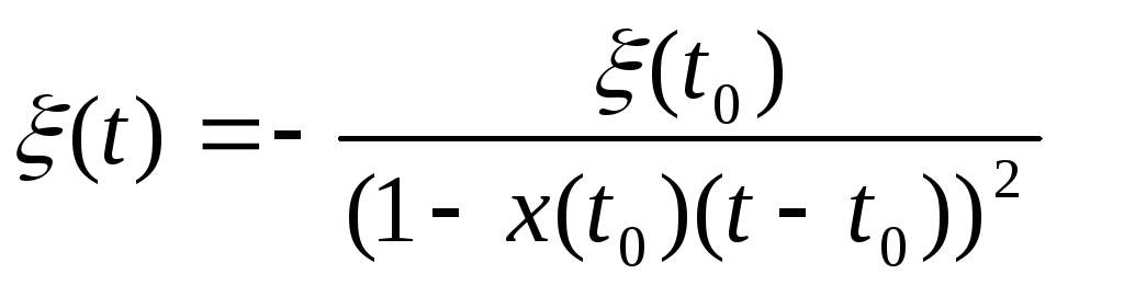 .
.
1.7. Typical disturbances
External disturbing influences can have a different character:
instantaneous action in the form of an impulse and constant action.
If we differentiate in time  , then
  , therefore(t) - function is a time derivative of a single step action.
(t) - the function during integration has the following filtering properties:
Integrable product of an arbitrary function  and(t) - filters out functions from all values
  only that which corresponds to the moment of application of an instantaneous single impulse.
|
Linear perturbation |
Harmonic perturbation
|

2 U. Second order systems
2.1 Reduction of second-order equations to systems of first-order equations
An example of a linear stationary system.
Another description of the same second-order system is given by a pair of coupled first-order differential equations
 (2)
(2)
where the relationship between the coefficients of these equations is determined by the following relations

2.2. Solution of second order equations
Applying the differential operator  the equation can be written in a more compact form
Equation (1) is solved in 3 stages:
1) find a general solution  homogeneous equation;
2) find a particular solution  ;
;
3) the complete solution is the sum of these two solutions  .
.
We consider the homogeneous equation
we will look for a solution in the form
 (5)
(5)
where  real or complex value. Substituting (5) into (4), we obtain
 (6)
(6)
This expression is a solution to a homogeneous equation if s satisfies the characteristic equation
For s 1 s 2, the solution of the homogeneous equation has the form
Then we look for a solution in the form  and substituting it into the original equation
Whence it follows that  .
.
If choose
 .
(8)
.
(8)
A particular solution of the original equation (1) is sought by the variation method  in the shape of

based on (11), (13) we obtain the system

Complete solution of the equation.


By changing variables, we obtain a second-order equation:

PHASE PLANE
A two-dimensional spatial state or phase plane is a plane in which two state variables are considered in a rectangular coordinate system
 - these state variables form a vector
  .
.
Schedule change  creates a trajectory. You must specify the direction of movement of the trajectory.
The state of equilibrium is called such a state  , in which the system remains, provided that
  The state of equilibrium can be determined (if it exists) from the relations

for any t.
Equilibrium states are sometimes called critical, main, or null points.
The trajectories of the system cannot intersect each other in space, which also follows from the uniqueness of the solution of the differential equation.
Not a single trajectory passes through the state of equilibrium, although they can approach singular points as close as they like (for  )
.
)
.
Point types
1 A regular point is any point through which the trajectory can pass, the equilibrium point is not regular.
2. An equilibrium point is isolated if its small neighborhood contains only regular points.
Consider the system

To determine the state of equilibrium, we solve the following system of equations
 .
.
Getting dependency between state variables  .
.
any point of which is a state of equilibrium. These points are not isolated.
Note that for a linear stationary system

the initial state turns out to be an equilibrium state and isolated if the determinant of the coefficient matrix 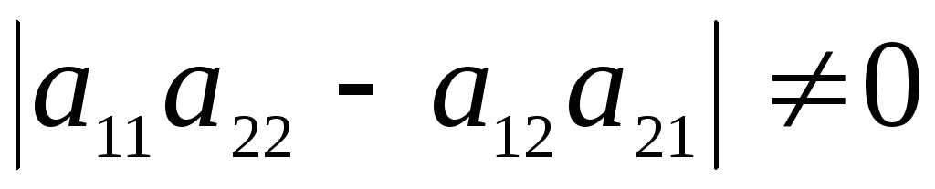 , then
  is a state of equilibrium.
For a non-linear system of the second order, the equilibrium state  called simple, if the corresponding Jacobi matrix is not equal to 0.

Otherwise, the state will not be simple. If the equilibrium point is simple, then it is isolated. The converse is not necessarily true (except in the case of linear stationary systems).
Consider the solution of the equation of state for a linear system of the second order:  .
.
This system can be represented by two first order equations,
denote  ,
,

Characteristic equation  and the solution will be:

The solution of the equation is written as

According to the nature of the functioning of the ACS, they are divided into 4 classes: Automatic stabilization systems are characterized by the fact that during the operation of the system the setting influence remains constant. Program control systems, the driving force changes according to a predetermined law as a function of time and coordinates of the system. Tracking systems, the driving force is a variable value, but the mathematical description in time cannot be established. Adaptive or self-adjusting systems, such systems automatically ...
Share work on social networks
If this work does not suit you, there is a list of similar works at the bottom of the page. You can also use the search button
Lecture number 2. Classification and Requirements for ATS. Linear and non-linear ACS. General Method linearization
(Slide 1)
2.1. ATS classification
(Slide 2)
ATS are classified according to various criteria. By the nature of the functioning of the ATS is divided into 4 classes:
- Systems automatic stabilization(characterized by the fact that the driving force remains constant during the operation of the system).Example: motor speed stabilizer.
- Systems program regulation(the master influence changes according to a predetermined law, as a function of time and coordinates of the system).Example: autopilot.
- Followers system (the master action is a variable value, but the mathematical description in terms of time cannot be established, since the signal source is an external action, the law of movement of which is not known in advance).Example: aircraft tracking radar.
- Adaptive or self-tuning systems (such systems automatically select the optimal control law and can change the characteristics of the regulator during operation).Example: a computer game with a non-linear plot.
(Slide 3)
ACS is also divided according to the nature of the signals in the control device:
- Continuous (input and output signal are continuous functions of time).Example: comparators, operational amplifiers.
- Relay (if the system has at least one element with a relay characteristic).Example: various relays, analog switches and multiplexers.
- Pulse (characterized by the presence of at least one impulse element).Example: thyristors, digital circuits.
All ACS can be divided according to the dependence of the output characteristics on the input into linear and non-linear.
2.2. Requirements for SAR
(Slide 4)
1. The controlled variable must be kept at the set level regardless of the disturbance. The transient process is represented by a dynamic characteristic, which can be used to judge the quality of the system.
2. The stability condition must be satisfied, i.e. the system must have a margin of stability.
3. Speed - the time of the transition process, which characterizes the speed of the system's response.
(Slide 5)
4. Overshoot regulations must be met. Two main parameters are used to determine the amount of overshoot:
- Overshoot factor
where y m is the maximum deviation of the output quantity during the transient, y∞ is the value of the output quantity in the steady state. Permissible value = 0 25%.
(Slide 6)
- The measure of the oscillation of the process is the number of oscillations during the transition process (no more than 2)
5. Must fulfill the requirement of static accuracy. If the processes in the system are random, then probabilistic characteristics are introduced to ensure accuracy.
2. 3 . Linear and non-linear ACS
Dynamic processes in control systems are described by differential equations.
(Slide 7)
In linear systems, processes are described usinglinear differentialequations. In nonlinear systems, processes are described by equations containing any non-linearity . Linear system calculations are well developed and easier to handle. practical application. Calculations of nonlinear systems are often associated with great difficulties.
In order for the control system to be linear, it is necessary (but not sufficient) to have the static characteristics of all links in the form of straight lines. In fact, real static characteristics in most cases are not straightforward. Therefore, in order to calculate the real system as a linear one, it is necessary to replace all the curvilinear static characteristics of the links in the working sections that are used in this control process with straight segments. It is called linearization . Most continuous control systems lend themselves to such linearization.
(Slide 8)
Linear systems are divided intoordinary linear systems and on special linear systems.The former include such systems, all links of which are described by ordinary linear differential equations with constant coefficients.
(Slide 9)
Special line systems include:
but) systems with time-varying parameters, which are described by linear differentialequations with variable coefficients;
b) systems with distributed parameters, where one has to deal with partial differential equations, and systems with a time delay described by equations with a retarded argument;
(Slide 10)
in) impulse systems, where one has to deal with difference equations.
(Slide 11)
Rice. 2.1. Characteristics of non-linear elements
In nonlinear systems, when analyzing the control process, it is necessary to take into account the non-linearity of the static characteristic in at least one of its links or some non-linear differential dependencies in the equations of the system dynamics. Sometimes non-linear links are specifically introduced into the system to provide the highest performance or other desired qualities.
Non-linear systems primarily include relay systems, sincerelay characteristic(Fig. 2.1, a and b ) cannot be replaced by a single straight line. A link will be non-linear, in the characteristic of which there isdead zone(Fig. 2.1, c).
Saturation phenomena or mechanical stroke limitationlead to a characteristic with limited linear dependence at the ends (Fig. 2.1, g ). This characteristic should also be considered non-linear if such processes are considered when the operating point goes beyond the linear section of the characteristic.
Non-linear dependencies also includehysteresis curve(Fig. 2.1, e ), characteristicclearance in mechanical transmission(Fig. 2.1, f), dry friction (Fig. 2.1, g), quadratic friction(Fig. 2.1, and ) and others. In the last two characteristics x 1 denotes the speed of movement, and x2 force or moment of friction.
Nonlinear is generally any curvilinear relationship between the output and input values of the link (Fig. 2.1, to ). These are nonlinearities of the simplest type. In addition, nonlinearities can enter differential equations in the form of a product of variables and their derivatives, as well as in the form of more complex functional dependencies.
Not all nonlinear dependencies lend themselves to simple linearization. So, for example, linearization cannot be done for the characteristics depicted in Fig. 2.1, but or in Fig. 2.1, f. Such complex cases will be considered in Sec. nine.
2.4. General linearization method
(Slide 12)
In most cases, it is possible to linearize non-linear dependencies using the method of small deviations or variations. To consider it, let's turn to a certain link in the automatic control system (Fig. 2.2). The input and output quantities are denoted by X 1 and X 2 , and external perturbation through F(t).
Let us assume that the link is described by some non-linear differential equation of the form
. (2.1)
To compile such an equation, you need to use the appropriate branch of technical sciences (for example, electrical engineering, mechanics, hydraulics, etc.) that studies this particular type of device.
(Slide 13)
The basis for linearization is the assumption that the deviations of all variables included in the link dynamics equation are sufficiently small, since it is precisely on a sufficiently small section that the curvilinear characteristic can be replaced by a straight line segment. The deviations of the variables are measured in this case from their values in the steady process or in a certain equilibrium state of the system. Let, for example, a steady process be characterized by a constant value of the variable X 1 , which we denote X 10 . In the process of regulation (Fig. 2.3) the variable X 1 will matter
where denotes the deviation of the variable x1 from the established value X 10.
Similar relationships are introduced for other variables. For the case under consideration, we have:
as well as
All deviations are assumed to be sufficiently small. This mathematical assumption does not contradict the physical meaning of the problem, since the very idea of automatic control requires that all deviations of the controlled variable during the control process be sufficiently small.
The steady state of the link is determined by the values X 10 , X 20 and F 0 . Then equation (2.1) can be written for the steady state in the form
. (2.2)
(Slide 15)
Let us expand the left side of equation (2.1) in the Taylor series
(2.3)
where are members of the highest order. The index 0 for partial derivatives means that after taking the derivative, the steady value of all variables must be substituted into its expression
; ; ; .
The higher order terms in formula (2.3) include higher partial derivatives multiplied by squares, cubes, and more high degrees deviations, as well as the products of deviations. They will be small of a higher order compared to the deviations themselves, which are small of the first order.
(Slide 16)
Equation (2.3) is a link dynamics equation, just like (2.1), but written in a different form. Let us discard the higher order smalls in this equation, after which we subtract the steady state equations (2.2) from Eq. (2.3). As a result, we obtain the following approximate link dynamics equation in small deviations:
(2.4)
In this equation, all variables and their derivatives enter linearly, that is, to the first degree. All partial derivatives are some constant coefficients in the event that a system with constant parameters is being investigated. If the system has variable parameters, then equation (2.4) will have variable coefficients. Let us consider only the case of constant coefficients.
(Slide 17)
Obtaining equation (2.4) is the goal of the linearization done. In the theory of automatic control, it is customary to write the equations of all links so that the output value is on the left side of the equation, and all other terms are transferred to the right side. In this case, all terms of the equation are divided by the coefficient at the output value. As a result, equation (2.4) takes the form
, (2.5)
where the following notation is introduced
(Slide 18)
In addition, for convenience, it is customary to write all differential equations in operator form with the notation
Etc.
Then the differential equation (2.5) can be written in the form
, (2.6)
This record will be called standard form records of the link dynamics equation.
Coefficients T 1 and T 2 have the dimension of time - seconds. This follows from the fact that all terms in equation (2.6) must have the same dimension, and for example, the dimension (or p x 2 ) differs from the dimension x 2 per second to the minus first power ( from -1 ). Therefore, the coefficients T 1 and T 2 are called time constants.
Coefficient k 1 has the dimension of the output value divided by the dimension of the input. It is calledtransmission ratiolink. For links whose output and input values have the same dimension, the following terms are also used: gain - for a link that is an amplifier or has an amplifier in its composition; gear ratio - for gearboxes, voltage dividers, scaling devices, etc.
The transfer coefficient characterizes the static properties of the link, as in the steady state. Therefore, it determines the steepness of the static characteristic at small deviations. If we depict the entire real static characteristic of the link, then linearization gives or. Transfer coefficient k 1 will be the tangent of the slope tangent at that point C (see Fig. 2.3), from which small deviations are counted x 1 and x 2 .
It can be seen from the figure that the linearization of the equation done above is valid for control processes that capture such a section of the characteristic AB , on which the tangent differs little from the curve itself.
(Slide 19)
In addition, another, graphical method of linearization follows from this. If the static characteristic is known and the point C , which determines the steady state, around which the regulation process takes place, then the transfer coefficient in the link equation is determined graphically from the drawing according to the dependence k 1 = tg c taking into account the scale of the drawing and dimensions x2 . In many casesgraphical linearization methodturns out to be more convenient and leads to the goal faster.
(Slide 20)
Coefficient dimension k2 equal to the dimension of the transfer coefficient k 1 multiplied by time. Therefore, equation (2.6) is often written in the form
where is the time constant.
Time constants T 1, T 2 and T 3 determine the dynamic properties of the link. This issue will be considered in detail below.
Coefficient k 3 is the transfer coefficient for external disturbance.
Page 1
Other related works that may interest you.vshm> |
|||
| 13570. | Linear and non-linear modes of laser heating | 333.34KB | |
| Linear regimes of laser heating To analyze the linear regimes of laser heating, we consider the processes of LR action on a half-space by a heat source exponentially decreasing with depth. Therefore, the idealization of the properties of heat sources, which is often allowed in calculation schemes to reduce mathematical difficulties, can lead to noticeable deviations of the calculated data from the experimental ones. For opaque materials, in most cases of LI heating, heat sources can be considered surface absorption coefficient α 104 105... | |||
| 16776. | Requirements for the tax policy of the state in a crisis | 21.72KB | |
| Requirements for the tax policy of the state in a crisis For the development of entrepreneurial activity in the current economic conditions, it is necessary to have certain conditions, including: - the presence of an effective tax system that stimulates the development of entrepreneurship; - the presence of a certain set of rights and freedoms, the choice of the type of economic activity, the planning of sources of financing, the access to resources, the organization and management of the company, etc. Thus, for the progressive development ... | |||
| 7113. | Harmonic linearization method | 536.48KB | |
| Method harmonic linearization Since this method is approximate, the results obtained will be close to the truth only if certain assumptions are met: A non-linear system must contain only one non-linearity; The linear part of the system should be a low-pass filter that attenuates the higher harmonics that occur in the limit cycle; The method is applicable only to autonomous systems. We study the free motion of the system, that is, the motion under non-zero initial conditions in the absence of external influences.... | |||
| 12947. | HARMONIC LINEARIZATION METHOD | 338.05KB | |
| Turning directly to the consideration of the harmonic linearization method, we will assume that the nonlinear system under study is reduced to the form shown in. A non-linear element can have any characteristic as long as it is integrable without discontinuities of the second kind. The transformation of this variable for an example by a non-linear element with a dead zone is shown in fig. | |||
| 2637. | Application medicines. General characteristics. Classification. Primary requirements. Technology of application of adhesives on a substrate in the production of application drugs | 64.04KB | |
| Application medicines - plasters corn adhesive plasters pepper plasters skin adhesives - liquid plasters TTC films, etc. General characteristics and classification of plasters Emplstr plasters a dosage form for external use that has the ability to stick to the skin, has an effect on the skin, subcutaneous tissues and in some cases a general effect on the body . Plasters are one of the oldest dosage forms known from very ancient times, the progenitors of modern drugs of the fourth generation... | |||
| 7112. | NONLINEAR SYSTEMS | 940.02KB | |
| The physical laws of motion of the world around us are such that all control objects are non-linear. Other non-linearities called structural are introduced into the system deliberately to obtain the required characteristics of the system. If the nonlinearities are weakly expressed, then the behavior of the nonlinear system differs slightly from the behavior of the linear system. It is impossible to create an exact model of a real system. | |||
| 21761. | The general pantheon of the gods of ancient Mesopotamia. Gods of ancient Sumer | 24.7KB | |
| The ancient religion of the peoples of Mesopotamia, despite its own conservatism, gradually, in the course of social development, underwent changes that reflected both the political and socio-economic processes taking place on the territory of Mesopotamia. | |||
| 11507. | formation of the financial result and general analysis of the financial and economic activities of the organization | 193.55KB | |
| For a deeper acquaintance with the activities of any enterprise, it becomes necessary to study it from all possible sides in the formation of the most objective opinion about both positive and negative aspects in work in identifying the most vulnerable places and ways to eliminate them. To conduct financial analysis, special tools are used, the so-called financial ratios. Using the necessary information to objectively and most accurately assess the financial condition of the organization, its profit and loss changes ... | |||
| 13462. | Statistical analysis of risky assets. Nonlinear Models | 546.54KB | |
| However, real data for many financial time series show that linear models do not always adequately reflect the true picture of price behavior. If we keep in mind the Doob decomposition in which conditional mathematical expectations are involved, it is quite natural to assume that the conditional distributions are Gaussian ... | |||
| 4273. | Linear mathematical models | 3.43KB | |
| Linear mathematical models. It was noted above that any mathematical model can be considered as some operator A, which is an algorithm or is determined by a set of equations - algebraic ... | |||
Function entry rules:
- All variables are expressed through x 1 ,x 2
- All mathematical operations are expressed through conventional symbols (+, -, *, /, ^). For example, x 1 2 +x 1 x 2 is written as x1^2+x1*x2 .
All the methods considered below are based on the expansion of a non-linear general function f(x) in a Taylor series up to first-order terms in the vicinity of some point x 0:
where ![]() is the discarded term of the second order of smallness.
is the discarded term of the second order of smallness.
Thus, the function f(x) is approximated at the point x 0 by a linear function:
,
where x 0 is the linearization point.
Comment. Linearization should be used with great care as it sometimes gives a very rough approximation.
General non-linear programming problem
Consider common task non-linear programming:
Let x t be some given estimate of the solution. Using direct linearization leads to the following problem:

This task is the PLP. Solving it, we find a new approximation x t +1 , which may not belong to the admissible region of solutions S.
If , then the optimal value of the linearized objective function that satisfies the inequality:
may not be an accurate estimate of the true value of the optimum.
For convergence to an extremum, it is sufficient that the sequence of points ( x t ) obtained as a result of solving the sequence of LP subtasks satisfies the following condition:
the value of the objective function and the constraint residual at the point x t +1 must be less than their values at the point x t .
Example #1. 
Let us construct an admissible region S (see the figure).

The admissible region S consists of the points of the curve h(x)=0 lying between the point (2;0) defined by the constraint x 2 ≥0 and the point (1;1) defined by the constraint g(x) ≥0.
As a result of the linearization of the problem at the point x 0 =(2;1), we obtain the following LLP:

Here it is a straight line segment bounded by the points (2.5; 0.25) and (11/9; 8/9). The level lines of the linearized objective function are straight lines with a slope of -2, while the level lines of the original objective function are circles centered at (0;0). It is clear that the solution of the linearized problem is the point x 1 =(11/9; 8/9). At this point we have:

so the equality constraint is violated. Having made a new linearization at the point x 1 , we get a new problem:

The new solution lies at the intersection of the lines ![]() and and has coordinates x 2 =(1.0187; 0.9965). Constraint - Equality (
and and has coordinates x 2 =(1.0187; 0.9965). Constraint - Equality ( ![]() ) is still violated, but to a lesser extent. If we make two more iterations, we get a very good approximation to the solution x * =(1;1), f(x *)=2
) is still violated, but to a lesser extent. If we make two more iterations, we get a very good approximation to the solution x * =(1;1), f(x *)=2
Table - Values of the objective function for some iterations:
| Iteration | f | g | h |
| 0 | 5 | 3 | –1 |
| 1 | 2,284 | 0,605 | –0,0123 |
| 3 | 2,00015 | 3.44×10 -4 | –1.18×10 -5 |
| Optimum | 2 | 0 | 0 |
It can be seen from the table that values f,g and h improve monotonically. However, such monotonicity is typical for problems whose functions are "moderately" non-linear. In the case of functions with pronounced nonlinearity, the monotonicity of the improvement is broken and the algorithm ceases to converge.
There are three ways to improve direct linearization methods:
1. Using a linear approximation to find the direction of descent.
2. Global approximation of the nonlinear function of the problem using a piecewise linear function.
3. Application of successive linearizations at each iteration to refine the allowable area S.
General linearization method
In most cases, it is possible to linearize non-linear dependencies using the method of small deviations or variations. To consider ᴇᴦο, let's turn to some link in the automatic control system (Fig. 2.2). The input and output quantities are denoted by X1 and X2, and the external perturbation is denoted by F(t).
Let us assume that the link is described by some non-linear differential equation of the form
To compile such an equation, you need to use the appropriate branch of technical sciences (for example, electrical engineering, mechanics, hydraulics, etc.) that studies this particular type of device.
The basis for linearization is the assumption that the deviations of all variables included in the link dynamics equation are sufficiently small, since it is precisely on a sufficiently small section that the curvilinear characteristic can be replaced by a straight line segment. The deviations of the variables are measured in this case from their values in the steady process or in a certain equilibrium state of the system. Let, for example, the steady process is characterized by a constant value of the variable X1, which we denote as X10. In the process of regulation (Fig. 2.3), the variable X1 will have the values where denotes the deviation of the variable X 1 from the steady value X10.
Similar relationships are introduced for other variables. For the case under consideration, we have ˸ and also .
All deviations are assumed to be sufficiently small. This mathematical assumption does not contradict the physical meaning of the problem, since the very idea of automatic control requires that all deviations of the controlled variable during the control process be sufficiently small.
The steady state of the link is determined by the values X10, X20 and F0. Then equation (2.1) should be written for the steady state in the form
Let us expand the left side of equation (2.1) in the Taylor series
where D are higher order terms. Index 0 for partial derivatives means that after taking the derivative, the steady value of all variables must be substituted into its expression.
The higher order terms in formula (2.3) include higher partial derivatives multiplied by squares, cubes and higher degrees of deviations, as well as products of deviations. They will be small of a higher order compared to the deviations themselves, which are small of the first order.
Equation (2.3) is a link dynamics equation, just like (2.1), but written in a different form. Let us discard the higher-order smalls in this equation, after which we subtract the steady-state equations (2.2) from Eq. (2.3). As a result, we obtain the following approximate equation of the link dynamics in small deviations˸
In this equation, all variables and their derivatives enter linearly, that is, to the first degree. All partial derivatives are some constant coefficients in the event that a system with constant parameters is being investigated. If the system has variable parameters, then equation (2.4) will have variable coefficients. Let us consider only the case of constant coefficients.
General linearization method - concept and types. Classification and features of the category "General linearization method" 2015, 2017-2018.
Statistical study of nonlinear systems is a very difficult task. The comparative simplicity of the methods of statistical analysis of linear systems is a natural reason for attempts to extend these methods to problems of approximate investigation of the accuracy of nonlinear systems. This is how methods of linearizing the nonlinear characteristics of systems arose.
The simplest form of linearization of nonlinear systems is linearization by expanding all nonlinear functions included in the equations of the system into a Taylor series and discarding all terms of the series above the first degree. In this case, each nonlinear function included in the equation of the system is replaced by an approximate linear expression
where is the mathematical expectation of the random function x.
A formula of the form (XVII.1) allows one to linearize the equations of a nonlinear system with respect to signal fluctuations in various elements of the system. This makes it possible to apply the methods statistical theory linear systems. However, formulas of the form (XVII. 1) are applicable only to continuous functions that have continuous derivatives with respect to the argument in the region of its practically possible values.
Meanwhile, automatic control systems often contain essentially non-linear links, the characteristics of which are discontinuous or have discontinuous derivatives. These characteristics include relay characteristics, limited linearity zones, etc. (see Book 1, Chapter IV). For the linearization of such characteristics, the method of statistical linearization was developed, .
Statistical linearization is the replacement of a non-linear link with a link that is linear with respect to fluctuations, while maintaining, in a certain sense, the level of the useful signal and the level of fluctuations at the output. In this case, the nonlinear function is approximated by a constant equivalent linear gain. Naturally, the approximation of nonlinear functions by a constant coefficient is not complete enough.
reflects the physical picture of the transformation of a random signal, since the transformation of the signal spectrum by a nonlinear link is not taken into account. In this regard, the paper proposed an approximation of inertialess nonlinear links by a statistically equivalent transfer function determined from the ratio of the spectral signal density at the output of the nonlinear link to the spectral signal density at the input.
At the same time, the statistical linearization of nonlinear functions was developed under the condition that the input signal contains a periodic component. This method was later called joint statistical and harmonic linearization.
The named methods of linearization make it possible to reduce the system of nonlinear differential equations to a system of linear equations, equivalent to the initial one in terms of the first two moments of the random function. Therefore, using the method of statistical linearization, it is possible to determine only the mean value and variance of a random function. When using joint linearization, it is also possible to determine the first harmonic of periodic oscillations in a nonlinear system.
Due to the fact that in a nonlinear system the probability density function of a random signal can differ significantly from the normal one, and in this case, to characterize the accuracy of operation, knowledge of only the first two moments is not sufficient in Ref. 113], a method of generalized statistically equivalent transfer function was developed, based on on the expansion in a series in orthogonal Chebyshev - Hermite polynomials of random functions and allowing to determine the highest moments of these functions in a nonlinear system.
The main idea of the statistical linearization method is to approximate essentially nonlinear transformations with a linearized dependence equivalent to a nonlinear transformation in the first two moments of random functions, i.e., in terms of the mean value and variance. Of course, this equivalent linearized dependence has a different form for different essentially non-linear elements, and also depends on the probabilistic characteristics of a random signal at the input of a non-linear element.
Consider a nonlinear transformation corresponding to the real static characteristic of a non-inertia non-linear element
The transformable random process can be represented as
where is the mathematical expectation, and is a process with zero mathematical expectation.
Let us represent the signal at the output of a non-linear element as an equivalent linear transformation of the input signal
where K - equivalent statistical transfer coefficients for mathematical expectation and dispersion, which must be determined. The first assumption, which is the starting point in determining these coefficients, is the observance of the equalities of the mathematical expectation and dispersion for a random signal at the output of a real non-linear and equivalent linear elements. Then the coefficient can be defined as the ratio of the mathematical expectation at the output of the nonlinear element to the mathematical expectation of the signal at the input
For the coefficient in this case, we will have the expression

where are the standard deviations of centered random signals, respectively, at the input and output of the nonlinear element.
The second assumption made in statistical linearization is based on the requirement that the mean square of the difference between the random signal at the output of a non-linear element and the random signal at the output of an equivalent linear element be minimum. This condition can be written as follows:
Let's expand this expression:
In the formula (XVI 1.8), the overline means the mathematical expectation. Taking the partial derivatives of the expression (XVI 1.8) with respect to we obtain

where is the mutual correlation function of the signals at the input and output of the equivalent linear element at
The use of the coefficient (XVI 1.6) in the calculations gives a somewhat overestimated value of the dispersion, and the use of the coefficient (XVI 1.9) somewhat underestimates. Therefore, when calculating, the following value can be taken as the equivalent coefficient for the random component:
![]()
Note that with statistical linearization, in contrast to the usual linearization of nonlinear functions based on their expansion in a Taylor series in the vicinity of a certain operating point, the average signal characteristics can be calculated exactly.
Now consider general formulas to determine the equivalent gains. Let a one-dimensional normal probability density be given). Then the formulas for the coefficients will look like

Let us calculate the coefficients using formulas (XVII.11), (XVII.12) and (XVII.13) for a nonlinear characteristic of the cubic parabola type, which can be analytically represented by the formula